1 Introduction and short recap of R
Goals: In this Lecture 1 we will give a introduction to the course and a short recap of using R.
1.1 Introduction
This course is called applied predictive modelling. What do we actually mean by these three words? Well, applied is as opposed to theoretical - indicating that this will not be a very theoretical course. We will focus on usage of the different methods that you will learn throughout the course. Predictive modelling means that the overall goal of the modelling is to predict something or make a prediction. Gkisser (1993) defines predictive modelling as “the process by which a model is created or chosen to try to best predict the probability of an outcome,” while Kuhn and Johnson (2016) define it as “the process of developing a mathematical tool or model that generates an accurate prediction” and the give the following examples of types of questions one could be interested in predicting:
- How many copies will a book sell?
- Will this customer move their buisness to a different company?
- How much will my house sell for in the current market?
- Does a patient have a specific disease?
- Based on past choices, which movies will interest this viewer?
- Should I sell this stock?
- Which people should we match in our online dating service?
- Is an email spam?
- Will this patient respond to this therapy?
Examples of stakeholders or users of predictive modelling can be insurance companies. They need to quantify individual risk of potential policy holders. If the risk is too high, they may not offer the potential customer insurance or they may use the quantified risk to set the insurance premium. Governments may use predictive models to detect fraud or identify terror suspects. When you go to a grocery store and sign up for some discounts, usually either by creating an account or registering your credit card, your purchase information is being collected and analyzed in an attempt to who you are and what you want.
Predictive modelling can often a good thing. When for instance Netflix learns what kind of TV-shows you prefer to watch, they can come up with suggestions for other TV-shows that you are likely to also enjoy. This can often be recognized by statements like “people who liked TV-series A, also liked TV-series B.” For the streaming provider the goal is to keep you as an entertained, satisfied and paying customer, but it is also in your interest to find entertainment that you like. But you have probably also noticed that sometimes, these predictions are quite inaccurate and provide the wrong answer. For instance, you did not like the suggested series or you did not receive an important email because it was wrongly classified as spam by (predictive) spam filter.
Kuhn and Johnson (2016) give four reasons for why predictive models fail:
- Inadequate pre-processing of the data.
- Inadequate model validation.
- Unjustified extrapolation.
- Over-fitting the model to existing data.
They also mention the fact that modellers tend to explore realtively few models when searching for predictive realationships. This is usually because the modeler has a preference for a certain type of model (the one he/she has used before and know well). It can also be due to software availability. We will cover (at least) some of these aspects in this course.
1.1.1 Prediction or interpretation?
In the examples listed above, the main goal is to predict something and there are likely data available to train a statistical model to do so in most of the cases. Note that we are not so interested in answering questions of why something happens or not. Our primary interest is to accurately predict the probability that something will, or will not, happen. In situations like these, we should not be worried with having interpretative models, and focus our attention on prediction accuracy. If your spam filter classifies an email as spam, you would not care why the filter did so, as long as you receive the emails you care about and not the ones you do not. An interpretative model can be a model for a certain stock’s value that can support statements like “the stock value prediction went up, because the company released information about a big contract.” One can explain why the model behaves the way it does. The alternative is often called a “black box,” meaning that you put your data in on one side of the box and on the other the prediction pops out, without you knowing what happened inside the box.
So, our primary interest is prediction accuracy. Cannot interpretability be our secondary target, so we can understand why it works? Kuhn and Johnson (2016) writes that “the unfortunate reality is that as we push towards higher accuracy, models become more complex and their interpretability becomes more difficult.”
1.1.2 Terminology
In the predictive modelling terminology there are quite a lot of things that mean the same thing. We will list some terminology here with some explanations (see Kuhn and Johnson (2016, p6)):
- The terms sample, data point, observation, or instance refer to a single, independent unit of data, e.g. a customer, a patient, a transaction, an individual. Sample can also refer to a collection of data points (a subset).
- The training set consists of data used to develop the models while the test and validation sets are used solely for evaluating the performance of the final model.
- The predictors, idendependent variables, attributes, descriptors, or covariates are the data used as input for the prediction equation (e.g. what you feed into the black box).
- Outcome, dependent variable, target, class, or response refer to the outcome of the event or qunatity that is being predicted (e.g. what comes out of the black box).
- Continuous data have natural, numeric scales (e.g. blood pressure, price of an item, a persons body mass index, number of bathrooms, etc).
- Categorical, nominal, attribute or discrete data all mean the same thing. These are data types that take on specific values that have no scale (e.g. credit status (“good” or “bad”) or color (“red,” “white,” “blue”))
- Model building, model training, and parameter estimation all refer to the process of using data to determine values of model equations.
1.2 Recap of R
1.2.1 Installing R and Rstudio
If you have not already installed the newest version of R and Rstudio on your personal computer, we will now tell you how. This installation guide will be based on Windows, but iOS and Linux are very similar and we will indicate where to deviate. The video below shows the same steps as listed.
First we install R:
- Go to https://cran.uib.no.
- Select Download R for Windows (or macOS/Linux) (this will be the newest R version).
- Go to your “Downloads” folder and run the .exe file.
- Use standard settings throughout the installation steps (click next-next-next-etc.).
- R is now installed.
Now that R is installed, we can install Rstudio:
- Go to https://www.rstudio.com/products/rstudio/download/.
- Press “Download” under the Rstudio Desktop - Open source licenece - Free.
- Press “Download Rstudio for Windows.” I guess if you have macOS/Linux it will detect that automatically. If not, select it manually from the list below.
- Go to your “Downloads” folder and run the Rstudio.exe file.
- Use standard settings throughout the installation steps (click next-next-next-etc.).
- RStudio is now installed.
Open RStudio and check that the print-out in the console matches the R version you just installed. At the time when this is written the newest version is 4.1.1 (2021-08-10) “Kick Things.” The printout at the top looks like this:
R version 4.1.1 (2021-08-10) – “Kick Things”
Copyright (C) 2021 The R Foundation for Statistical Computing
Platform: i386-w64-mingw32/i386 (32-bit)
If you had R and Rstudio already, but updated to the newest version, remember that you will have to also install all your packages again.
1.2.2 R community and packages
Currently, there are over 18 000 packages available on the official CRAN server - open source and free. If you have a problem and need a smart function for solving that, you will most likely find that someone else have had the same problem, already solved it and made an R package that you can use. The large R community is also very active on the net forum stackexchange.com. If you have a programming issue and google it, you will typically end up in one of these forums where someone else has posted a question similar to yours and others from the community has provided a solution. I have been using R for over 10 years now and this strategy for solving programming issues has not failed me yet.
Once you have found an R package you want to install, you can install it using the install.packages function. We will use the tidyverse package developed by Wickham et al. (2019) as an example. This is a bundling package built up of many packages, which we will use throughout the course.
install.packages("tidyverse")To load a package into you R environment, making all its functionality available to you, you can use the library or require functions. The two are quite equal, but if you do not have the package installed require will cast a warning and continue, while library will cast an error and stop.
library(tidyverse)As part of the output here, you can see all the packages that tidyverse attaches to your working environment. We will be using many of these.
1.2.3 Datacamp
As a part of the course, you will be given access to Datacamp. We will suggest courses to take there in combination with the lectures provided.
If you want a more thorough recap of using R, you can take the course Introduction to R or test yourself with the practice module Introduction to R.
1.3 Data preprocessing
Data pre-processing techniques typically involve addition, deletion or transformation of training set data. Preparing the data in a good way can make or break the predictive ability of a model. How the predictors enter the model is important. By transforming the data before feeding them to the model one may reduce the impact of data skewness or outliers. This can signifcantly improve the model’s performance. The need for data pre-processing may depend on the method you are using. A tree-based model is notably insensitive to the characteristics of the predictor data, while a linear regression is not.
How the predictors are encoded, called Feature engineering, can also have a huge impact on the model performance. There are many ways to encode the same information. Combining multiple predictors can sometimes be more effective than using the individual ones. For example, using the body mass index (BMI = weight/length\({}^2\)) instead of using length and weight as separate predictors. The modeler’s understanding of the problem can often help in choosing the most effective encoding.
Different ways of encoding a date predictor can be
- The number of days since a reference date
- Using the month, year and day of the week as separate predictors
- The numeric day of the year (julian day)
- Whether the date was within the school year (as opposed to holiday)
1.4 Case study
We will use the same example as Kuhn and Johnson (2016) from the R package
install.packages("AppliedPredictiveModeling")1.4.1 Data transformations for individual predictors
library(AppliedPredictiveModeling)
data("segmentationOriginal")
segData <- subset(segmentationOriginal, Case == "Train")
1.4.2 Centering and scaling
The most straightforward and common transformation of data is to center and scale the predictor variables. Let \(\textbf{x}\) be the predictor, \(\overline{x}\) its average value and \(sd(x)\) it’s standard deviation. Centering means to substract the average predictor value from all the predictor values (\(\textbf{e} = \textbf{x}-\overline{x}\)) and scaling means dividing all values by the empirical standard deviation of the predictor (\(\textbf{e}/sd(x)\)). By centering the predictor, the predictor has zero mean and by scaling, you coerce the value to have a common standard deviation of one. A common term for a centered and scaled predictor is a standarized predictor, indicating that if you do this to all predictors they are all on a common scale. In the Figure 1.1 below, we have simulated 1000 normally distributed observations with mean 22 and standard deviation 4 and plotted a histogram of them (left panel) and a histogram of them standardized (right panel). As you can see, the distribution looks the same, but the scale on the x-axes has changed.
library(ggplot2)
set.seed(123)
x <- rnorm(1000, mean = 22, sd = 4)
df <- data.frame(x = c(x, (x-mean(x))/sd(x)),
                 mean = rep(c(22, 0),each = 1000),
                 type = rep(c("Original", "Standardized"), each = 1000))
ggplot(data= df,aes(x = x, fill = type)) +
  geom_histogram() +
  facet_wrap(~type, scales = "free") +
  geom_vline(aes(xintercept = mean), col = 1, lty = 2) +
  scale_y_continuous(expand =c(0,0)) +
  theme(legend.title = element_blank(),
        legend.position = "none")+
  xlab("")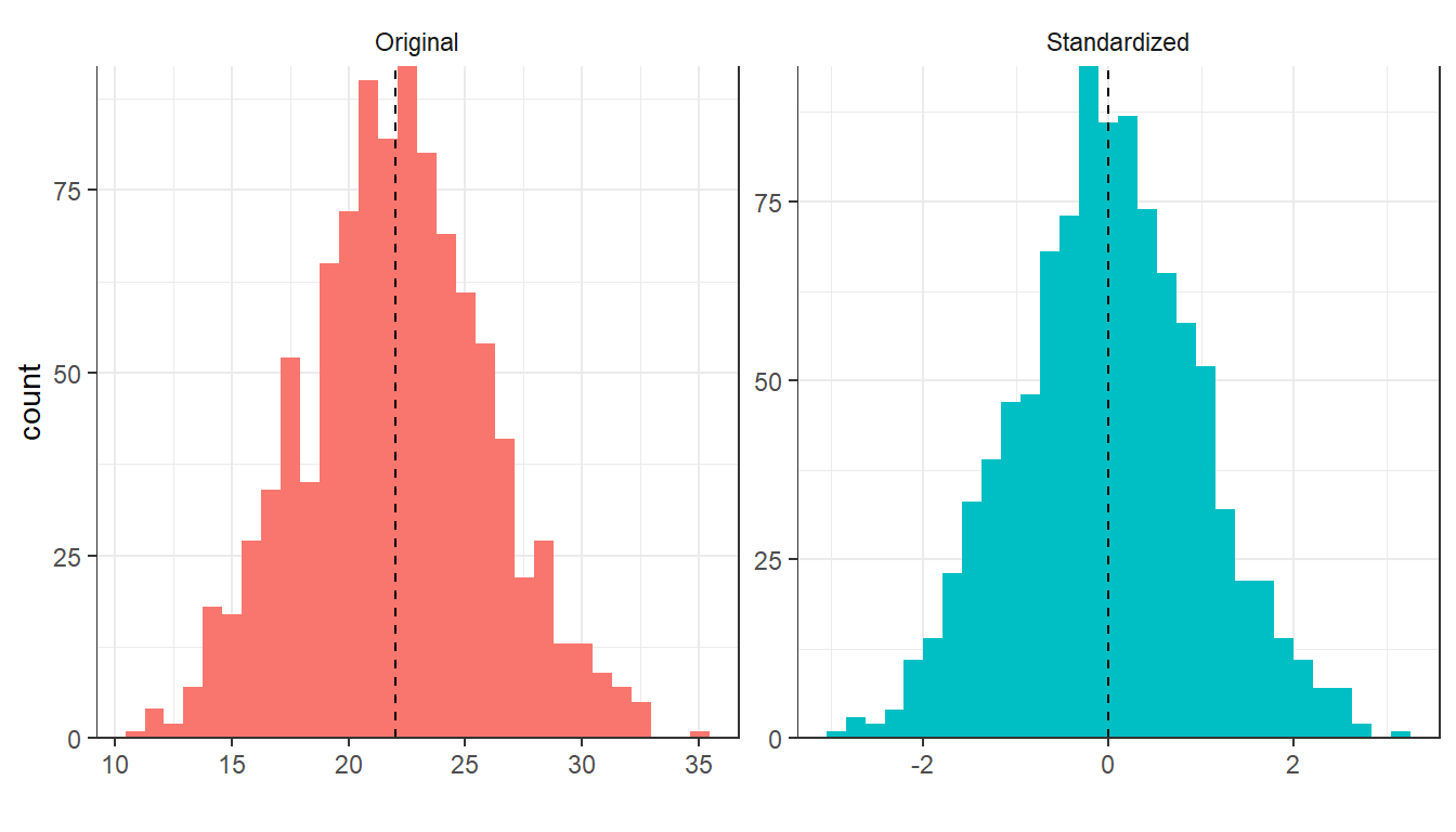
Figure1.1: Simulated normally distributed variables on original- and standardized scale.
1.4.3 Tranformations to resolve skewness
As noted above, standardizing preserves the distribution, but sometimes we need to remove distributional skewness. An un-skewed distribution is roughly symmetric around the mean. A right-skewed distribution has a larger probability of falling on the left side (i.e. small values) than on the right side (large values). We have illustrated left-, right- and un-skewed normal distributions in Figure 1.2.
x <- seq(-4,4,by = .1)
alpha <- c(-5,0,5)
df <- expand.grid("x" = x,"alpha" = alpha)
df <- df %>% mutate(case = ifelse(alpha == -5, "Left skewed",
                                  ifelse(alpha ==5, "Right skewed",
                                         "Unskewed")),
                    delta = alpha/sqrt(1+alpha^2),
                    omega = 1/sqrt(1-2*delta^2/pi),
                    dens = sn::dsn(x,xi = -omega*delta*sqrt(2/pi),  alpha =alpha, omega = omega))
ggplot(df, aes(x = x,y = dens)) +
  geom_line() +
  facet_wrap( ~case, scales = "fixed", nrow = 3, strip.position = "right") +
  geom_vline(xintercept = 0, lty = 2) +
  xlab("") + ylab("Density")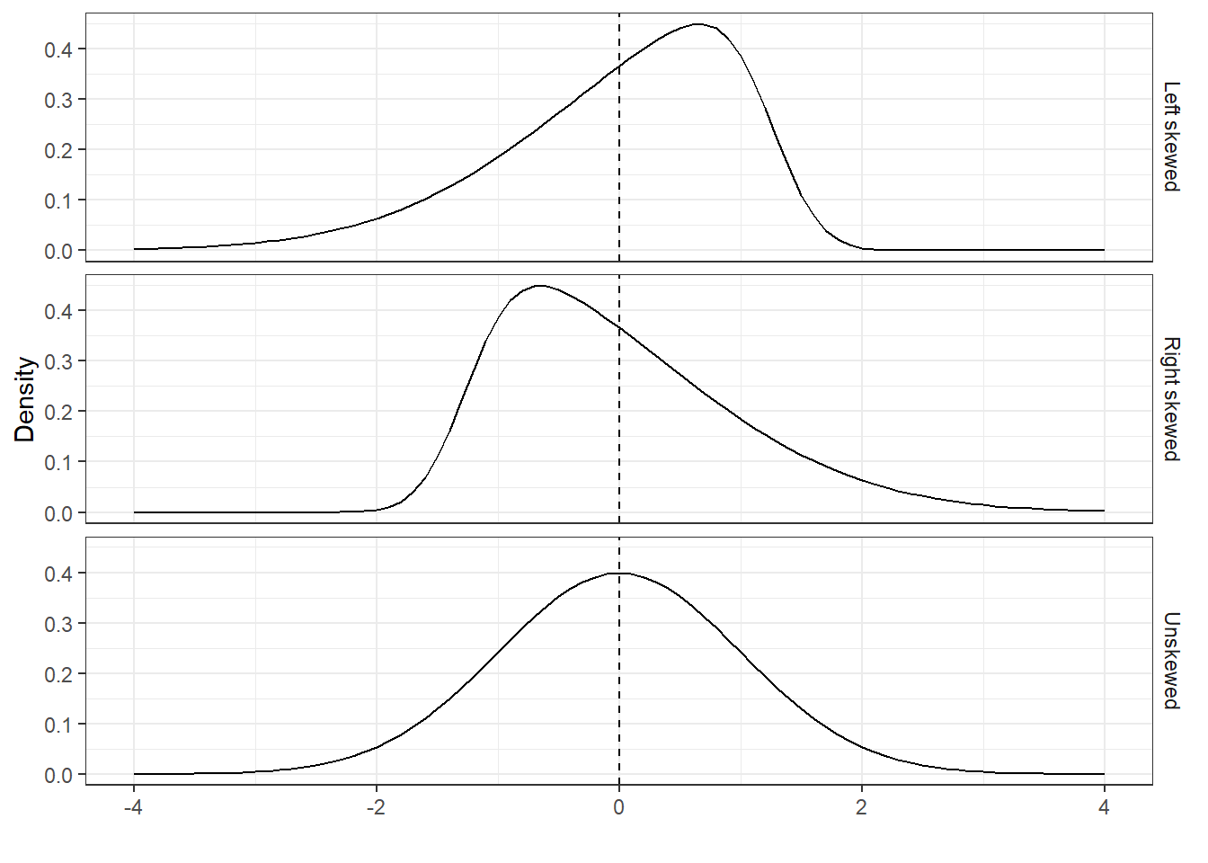
Figure1.2: Skewed normal distributions with mean 0 and standard deviation 1.
A rule of thumb to consider is that skewed data whose ratio of the highest value to the lowest value is greater than 20 have significant skewness. One can calculate the skewness statistic and use that as a diagnostic. Is it close to zero, the distribution if roughly symmetric. Is it large, indicates right-skewness and negative values indicates left-skewness. The formula for the sample skewness statistic is given by
\[\text{skewness} = \frac{\sum_{i=1}^n (x_i-\overline{x})^3}{(n-1)v^{3/2}},\quad \text{where}\quad v = (n-1)^{-1}\sum_{i=1}^n(x_i-\overline{x})^2,\]
\(x\) is the predictor variable, \(n\) the number of values and \(\overline{x}\) is sample mean.
Transforming the predictor with the log, square root or inverse may help remove the skew. Alternatively, a Box-Cox transformation can be used. The Box-Cox family of transformations are indexed by a parameter denoted \(\lambda\) and defined by
\[x^\star = \begin{cases} \frac{x^\lambda-1}\lambda, & \text{if }\lambda\neq 0\\ \log(x), & \text{if }\lambda = 0. \end{cases}\]
In addition to the log transformation, the family can identify square transformation (\(\lambda = 2\)), square root (\(\lambda = 0.5\)), inverse (\(\lambda = -1\)) and other in-between. By using maximum likelihood estimation on the training data, \(\lambda\) can be estimated for each predictor that contain values greater than zero.