8 Artificial Neural networks
This section describes the basics theory and classical optimization of an artificial neural network. This includes defining a 2-layer feed forward neural network, cost and objective functions, regularization and the manner in which a network can be trained to produce desired output. The section will be limited to so-called supervised learning, i.e. where know the true state of an output. The main references for this chapter are the textbook “Deep Learning” by @{goodfellow2016deep}.
8.1 Feed Forward Neural Networks
Let \(\mathbf{X}^{(i)}\) be an instance of data which is input to a deep learning model, with associated target values \(\mathbf{y}^{(i)}\). A target value can be a class or as we will use later the data \(\mathbf{X}^{(i)}\) itself. All the instances of \(\mathbf{X}^{(i)},\) \(i=1, \ldots N,\) constitute the data set \(\mathbf{X}^{(i)}\), and all the target values \(\mathbf{y}^{(i)},\) \(i=1, \ldots N,\) comprise the data set \(\mathbf{Y}\).
A feed forward neural network is a hierarchical model that consists of nodes or computational units divided into subsequent layers. For each node, a non-linear activation function is applied. The nodes between each layer are connected, so that the input to a node is totally dependent on the output from the nodes of the previous layer. The model is called a deep learning model if there are multiple hidden layers; see @ref(#fig:NN_model). The simplest deep learning model has at least one hidden layer: an input layer and an output layer. This hierarchical structure makes it possible to formulate the deep learning model as a linear system of equations.
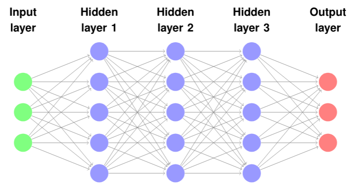
Illustration of a deep neural network with three hidden layers
The model input to a neural network is here defined as vector \(\mathbf{x}^{(i)}\) with \(Q\) elements. The input is transformed linearly by \(\mathbf{W}_1\) and \(\mathbf{b}\) such that \(f(\mathbf{x}^{(i)}) = \mathbf{W}_1 \mathbf{x}^{(i)} + \mathbf{b}\). \(\mathbf{W}_1\) transforms the input to a vector of \(K\) elements and is often called the weight matrix, while the translation \(\mathbf{b}\) is referred to as the bias. The bias can be interpreted as a threshold for when the neuron activates.
A nonlinear activation function is applied element wise to the transformed data. The activation function is typically given as a rectified linear unit (ReLU) @{nair2010rectified} \(Relu(z) = max(0, z)\) or \(\tanh\) function. This activation introduces non-linearity to the other linear operations. The superposition of the linear and nonlinear transformation is in combination with the activation function and is what we refer to as a hidden layer.
Applying another linear transformation \(\mathbf{W}_2\) to the hidden layer results in this case to the model output or output layer. The size of the output layer is a row vector with \(D\) elements. Generally, many transformations and activations can be applied consecutively which will result in a more complex hierarchical model. A generalization to a network with several hidden layers is straightforward; to make this clear we here limit the notation to a single hidden layer. We note that \(\mathbf{x}^{(i)}\) is vector of size \(Q\), \(\mathbf{W}_1\) is a \(K \times Q\) matrix that transforms the input to \(K\) elements, \(\mathbf{W}_2\) is a \(D \times K\) matrix, transforming the vector into \(D\) elements and \(\mathbf{b}\) consists of \(K\) elements. We write this as linear system of equations transformed with the activation function \(\sigma\)
\[\widehat{\mathbf{y}}^{(i)} = \mathbf{W}_2 (\sigma(\mathbf{W}_1 \mathbf{x}^{(i)} + \mathbf{b})) := \mathbf{f}^{\omega}, \qquad \omega = \{\mathbf{W}_1, \mathbf{W}_2, \mathbf{b}\}\] Depending on how the output layer is defined, we can use the network for classification or regression tasks. For classification purposes, the number of nodes in the output layer equals the number of classes, and typically transformed with a softmax function @{goodfellow2016@softmax}. The softmax function is a generalization of the logistic map that normalizes the output relative to the different classes:
\[ \sigma(z_i) = \frac{e^{z_{i}}}{\sum_{j=1}^K e^{z_{j}}} \ \ \ for\ i=1,2,\dots,K \]
In regression problems we want to estimate relations between variables; we want to predict a continuous output based on some input (variables). To use a linear activation function on the output layer will serve this purpose.
It has been shown that ANN is a universal approximation @{hornik1989multilayer}; thus, our goal is to find the weights of the given network to best approximate the map from the input to the output. This means that we want to estimate the weights of the ANN \(\mathbf{\omega}\), given the input data \(\mathbf{x}^{(i)}\), the target \(\mathbf{y}^{(i)}\) such that the predictions \(\widehat{\mathbf{y}}^{(i)}\) is minimized towards the true target values \(\mathbf{y}^{(i)}\). This is a typical optimization problem, which can be minimized with an objective function and optimization procedure.
8.2 Objective functions and training
An objective function for use in deep learning typically contains two terms: cost function and regularization. The cost function takes the predicted and the true values as input. Depending on the task and what one wants to minimize, the cost function maximizes a likelihood. In classification problems this is often the negative cross entropy
\[\mathcal{C}_1^{\mathbf{W}_1, \mathbf{W}_2, \mathbf{b}}(\mathbf{X},\mathbf{Y}) = - \frac{1}{N}\sum\limits_{j=1}^{N}\mathbf{y}^{(i)}_j\log(\widehat{\mathbf{y}}^{(i)}_j) = -\log p(\mathbf{Y}|\mathbf{f}^{\mathbf{\omega}}(\mathbf{X})),\] and in regression problems the Mean Squared Error (MSE)
\[\mathcal{C}_2^{\mathbf{W}_1, \mathbf{W}_2, \mathbf{b}}(\mathbf{X},\mathbf{Y}) = \frac{1}{N}\sum\limits_{i=1}^{N}(\mathbf{y}^{(i)} - \widehat{\mathbf{y}}^{(i)})^2 = - \log p(\mathbf{Y}|\mathbf{f}^\mathbf{\omega}(\mathbf{X})),\]
Minimization of the negative cross entropy and the MSE is well known to be equivalent to minimize the negative log likelihood of the parameter estimation @{tishby1989consistent} for neural networks. Depending on the task, minimizing the cross entropy or the MSE with respect to the parameters \(\omega = \{\mathbf{W}_1, \mathbf{W}_2, \mathbf{b}\}\) maximizes the likelihood of these parameters. The choice of the cost function is not restricted to those given above, and depend on the data, the model structure and what one wants to predict with the model.
One of the key problems in deep learning is a phenomenon called over-fitting (See also Lecture 2). Over-fitting occurs if the optimized model performs poorly on new unseen data, i.e. it does not generalize well. To address this problem, regularization is added to the cost function.
Regularization is a general technique, where the goal is to make an ill posed problem well-posed. Over-fitting is basically one example of an ill-posed problem. For optimization problems, you could add a penalizing functional: L2 or L1 norm for the parameters; or use dropout @{srivastava2014dropout}.
Regularization in neural networks work by penalizing the cost function, e.g. forcing the weights to become small. The idea behind a specific regularization term could be to minimize the weights of the ANN to generate a simpler model that helps against over-fitting. \(L2\) regularization multiplied with some penalizing factor \(\lambda_i\) is one of the most common regularization techniques. The cost function with regularization is called the objective function. Adding \(L2\) regularization to the cross entropy or MSE result in the objective function
\[\mathcal{L}(\mathbf{W}_1, \mathbf{W}_2, \mathbf{b}) = \mathcal{C}^{\mathbf{W}_1, \mathbf{W}_2, \mathbf{b}}(\mathbf{X},\mathbf{Y}) + \lambda_1||\mathbf{W}_1||^2 + \lambda_2||\mathbf{W}_2||^2 + \lambda_3||\mathbf{b}||^2\]
Another common way of regularizing the cost function is through dropout, which is a stochastic regularization technique. In the example later we will utilize dropout as regularization. Minimizing the objective function with respect to the weights \(\mathbf{\omega}\) with a gradient descent optimization method has proven to give good results in a wide range of applications. The gradient descent method @{curry1944method} updates the parameter \(\mathbf{\omega}\) using the entire data set
\[\mathbf{\omega}_t = \mathbf{\omega}_{t-1} - \eta \nabla \mathcal{L}(\mathbf{\omega}_{t-1}). \]
Here \(\omega_t\) represents the current configuration of the weights, while \(\omega_{t-1}\) represents the previous one. The parameter \(\eta\) is referred to as the learning rate, i.e. how large the step in the negative gradient direction the update of the weights should be. Too small steps can lead to poor convergence, while to large steps can lead to overshooting, i.e. missing local/global minimums. Usually it is too expensive to calculate the gradient over the entire dataset. This is solved by a technique called stochastic gradient descent @{robbins1951stochastic}. Stochastic gradient descent performs a parameter update for each training example. A natural extension and a more cost-efficient approach is the mini-batch gradient descent approach. In mini-batch optimization, the gradient is approximated by calculating the mean of the gradients on sub-sets or batches of the entire data set,
\[\mathbf{\omega}_t = \mathbf{\omega}_{t-1} - \frac{\eta}{n}\sum\limits_{i=1}^{n}\nabla \mathcal{L}_i(\mathbf{\omega}_{t-1}).\]
The mini-batch gradient descent iterative process can be implemented in the neural network with the back-propagation algorithm @{rumelhart1988learning}. In back-propagation, the weights are updated through a forward and backward pass. In the forward pass, we predict with the current weight configuration and compare towards the target values. In the backward pass, we use the chain rule successively from the output to the input to calculate the gradient of \(\omega\). Based on the gradient direction and the learning rate, the configuration of the weights is updated.
To find the correct learning rate is difficult, hence, several methods has been developed to adjust the learning rate adaptively. One of the disadvantages of the vanilla gradient descent approach to the ANN optimization problem, is that it has a fixed learning rate \(\eta.\) In line with the development of ANN, methods dedicated to deep learning and adaptive adjustment of the learning rate have been developed. Besides SGD with momentum @{sutskever2013importance}, the two most used optimization methods for ANNs are ADAM @{kingma2014adam} and Root Mean Square Propagation (RMSProp) @{tieleman2012lecture}. RMSProp adaptively adjusts the learning rate of the gradients based on a running average for each of the individual parameters. The ADAM-algorithm individually adjusts the weights in terms of both the running average, but also with respect to the running variance.
The use of back-propagation together with a stochastic gradient descent method, increase in available data and hardware have been the successes of deep learning during the past decade.
8.3 Validation of trained models
To validate and ensure that the predictions of the deep learning model also performs well on new unseen instances, the data is split into three independent sub-data sets: a training, a validation and a test data set. The training data set is directly used to optimize the parameters of the model. The validation data set is indirectly used to optimize the model, that is, we monitor the performance on the validation dataset after each epoch. An epoch is one pass in the optimization over the entire training dataset. During training, the model sees the same training data multiple times, however, the instances are usually randomly shuffled before a new epoch starts.
After each epoch, we predict with this temporally model on the validation data set. Usually we put criteria on the performance on the validation data set for when to stop the optimization. We can use a so called early stopping regime, where the model stops training if it does not see improvement on the validation score after a certain number of epochs without improvement.
The purpose of the test data set is to validate on new unseen data that has not been part of the training or the continuous validation of the model. Lets look at an example of how to implement a classifier on the mnist data set in keras.
8.4 Implementation of Feed Forward Neural Network in Keras
In this section we will show you how to implement a Feed Forward Neural Network with dropout as regularization with the high level API for tensorflow called Keras. A lot of the development within deep learning is concentrated around the python programming language. Keras is also a tool that is originally developed in python, but also available in R. Lets start by installing tensorflow:
8.4.1 Installing Keras and Tensorflow
For people who use Windows you must install miniconda first. You can do this through the reticulate package (The reticulate package provides a comprehensive set of tools for interoperability between Python and R.). You can install reticulate and subsequently miniconda with the following commands:
install.packages("reticulate")
reticulate::install_miniconda()
If you have a linux or mac operating system, you should be able to run the subsequent commands directly. This is because you have python already installed on your computer. You can now install tensorflow with the following commands:
install.packages('tensorflow')
library('tensorflow')
install_tensorflow()
Then install keras with the following commands:
install.package('keras')
library(keras)
install_keras()
8.4.2 Importing MNIST
We will use the famous MNIST data set @{deng2012mnist} as an example in this section. The MNIST dataset contains 60000 handwritten digits for training the model, and 10000 for testing. The digits has a shape of 28x28 pixels in grey scale, that is, they only have one channel, describing the black/white intensity of the pixel value. Each picture/instance is associated with a label, that is a number from 0-9. The keras package contains a function for downloading the MNIST dataset from the source.
library(keras)
mnist <- dataset_mnist()
To ensure that the predictions of the neural network model also performs well on new unseen instances, the data is often split into three independent sub-data sets: a training, a validation and a test data set. The training data set is directly used to optimize/train the parameters of the model. The validation data set is indirectly used to optimize the model, that is, we monitor the performance on the validation dataset after each epoch. An epoch is one pass in the optimization over the entire training dataset. During training, the model sees the same training data multiple times, however, the instances are usually randomly shuffled before a new epoch starts. We will come back to validation and testing of the neural network later in this section. The MNIST dataset are split into a test and train data set from source
#
x_train <- mnist$train$x
y_train <- mnist$train$y
x_test <- mnist$test$x
y_test <- mnist$test$y
We can check out some of the training data
#checking the dimension of the train/test data
library(ggplot2)

# visualize the digits
par(mfcol=c(5,5))
par(mar=c(0, 0, 3, 0), xaxs='i', yaxs='i')

for (idx in 1:25) {
    im <- x_train[idx,,]
    im <- t(apply(im, 2, rev))
    image(1:28, 1:28, im, col=gray((0:255)/255),
          xaxt='n', main=paste(y_train[idx]))
}
#checking the dimension of the train/test data
dim(y_train)
head(y_train)Here we see that the training dataset has a shape of \(60000 \times 28 \times28\). This means that there are \(60000\) instances, or pictures of handwritten digits, where each of the pictures has \(28 \times 28\) dimension in the horizontal and vertical direction. The dimension of the y_train variable represents the class or label of the x_train variable.
8.4.3 Pre-processing
Pre-processing is the step where we transform, scale, removes, imputes etc. the data before we feed it to the deep learning model. Removing erroneous data, or impute NA values may be of crucial importance to get the algorithm run at all. Transforming or scaling the data helps improve the so called conditioning problem. Conditioning of a problem say something about the sensitivity of the solution to changes in the problem data. To create an easier problem to optimize, we pre-process the MNIST-data before we are feeding it to the neural network model. Here we reshape and scale the data.
# reshape
x_train <- array_reshape(x_train, c(nrow(x_train), 784))
x_test <- array_reshape(x_test, c(nrow(x_test), 784))
# rescale
x_train <- x_train / 255
x_test <- x_test / 255
We also need to convert the y_train and y_test to categorical variables. Instead of having a vector with a number from 0-9, we convert it to a binary representation. That is, each label is represented by a vector of length 10 with one element is 1 and the rest 0. The element that is 1 represent the label of the digit.
y_train <- to_categorical(y_train, num_classes = NULL)
y_test <- to_categorical(y_test, num_classes = NULL)

head(y_train)
8.4.4 Feed Forward Neural Network model
In this example we want to create a so called dense neural network, or feed forward neural network. That is, each node are influenced from all of the nodes in the previous layer. This is contrast to e.g. convolutional neural networks that uses convolutions to reduce the connectivity between layers, thus reducing the connections.
We construct a dense neural network. After reshaping the input, the network has a shape of \(28 \times 28 = 784\) per instance. This is our input shape. This shape has to be specified in the model, as shown below. The first layer has \(256\) nodes, and we use the rectified linear unit as activations function. The next layer is a so called dropout layer. This layer drops randomly a proportion of the nodes out during a forward and backward pass. This will help avoiding overfitting, i.e. it is a form of regularization of the network. The next hidden layer has \(128\) nodes, and also ReLU activation function. The last layer of the network is the output. The output in this case, is to classify the label of the digit. There are 10 possible classes, 0-9 and we thus use a softmax activation function, with 10 units.
model <- keras_model_sequential()
model %>%
  layer_dense(units = 256, activation = 'relu', input_shape = c(784)) %>%
  layer_dropout(rate = 0.4) %>%
  layer_dense(units = 128, activation = 'relu') %>%
  layer_dropout(rate = 0.3) %>%
  layer_dense(units = 10, activation = 'softmax')
First we construct a sequential model object. Then we can use the pipe syntax to specify the layers of the neural network. We can use the summary function to show a nice overview of the neural network model.
summary(model)8.4.5 Compiling and training the model
We now have a model, the next step is to compile it. Durring compiling we also have to specify the loss function, optimizer and metrics for evaluations and validation.
model %>% compile(
  loss = 'categorical_crossentropy',
  optimizer = 'adam',
  metrics = 'accuracy'
)
Since we want to classify the digits, we have chosen the loss to be categorical cross entropy. We use the adam-algorithm during optimization and we also specify that we want to return the accuaracy of the classification during training and validation.
After the compilation, we can call the fit() function to train our model. The fit function take x_train and y_train as inputs. We also have to specify how many epoch the model should be trained on (how many times we will see the entire data set), the batch size (how many/large the splits of the training data set) and how large proportion of the data should be used as online validation data. Test data are set aside for evaluation the model when it has finished training.
history <- model %>% fit(
  x_train, y_train,
  epochs = 30,
  batch_size = 128,
  validation_split = 0.2
)
It is possible to specify specific validation data if that is desirable. Batch size, epochs, size of the neural network, e.g. number of layers nodes, type of network (e.g. cnn, rnns) are so called hyper parameters. This is parameters that are not optimized in the network itself, but has to be specified manually. Theses hyper parameters are important and there are different strategies for optimize them. Hyper parameter search could be done with traditional grid search, but also more sophisticated approaches such as Bayesian hyper optimization.
We have plotted the loss and accuracy calculated after each training epoch. It can be observed that the loss after approx 10-15 epochs, is significantly lower than the validation loss. This is an indication that the model starts to overfit.
8.4.6 Evaluating the model
To evaluate the trained model on the test data, we can use the pipe syntax together with the evaluate function
model %>% evaluate(x_test, y_test)The trained model perform pretty well on the test data set. It has an accuracy of approximatley 0.98, that is 98 \(\%\) of the data in the test data set is classified correctly.
8.4.7 Predicting with the model
We can also predict the most probable class for each of the instances. For this we can use the predict function.
#model %>% predict(x_test) %>% k_argmax()
prediction <- model %>% predict(x_test)
#plot(prediction[1710,], )
dim(prediction)
Lets find someof the most uncertain predictions and plot them. We find the most probable predictions in the test data set, then we choose the predictions which has the lowest confident.
largest <- apply(prediction,1,max,na.rm=TRUE)
less_confident <- sort(largest,index.return = TRUE)$ix[1:36]
pred_class <- prediction %>% k_argmax()
Lets plot some of predictions with lowest confident
#and plot the digits
par(mfcol=c(6,6))
par(mar=c(0, 0, 3, 0), xaxs='i', yaxs='i')

for (idx in less_confident) {
    im <- mnist$test$x[idx,,]
    im <- t(apply(im, 2, rev))
    image(1:28, 1:28, im, col=gray((0:255)/255),
          xaxt='n', main=paste(mnist$test$y[idx]))
}
By visual inspection of the plot it`s understandable that the classifier has difficulties (at least some of them) with determine the correct class label of the pictures.
Data camp
We highly recommend the data camp course Introduction to TensorFlow in R chapters 1-3.