stationarity

We return to Labarr’s time series in 5 minutes series on youtube explaining stationarity. This is a key concept in time series. The video by Labarr gives a nice intuition for the concept. It separates between strong and weak stationarity. In this course, the weak stationarity condition will be the one we focus on, but it is nice to know that there are other definitions of stationarity as well. For a time series to be (weakly) stationary the mean and variance of the time series variable Y_t should not depend on t. More formally, a time series is weakly stationary if

The expectation is constant: \mu_t = \mu
The variance is constant and finite: \sigma_t^2 = \sigma^2 < \infty
The covariance between two lagged variables only depend on the lag: \gamma(r,s) = \gamma(h), where h=|r-s|.

In the video, Labarr shows some examples of non-stationary time series which can be transformed to stationary time series by differencing. We will come back to this later in the course, when we talk about transformations and again when we study ARIMA models. We will also study examples of stationary time / non-stationary time series in the voluntary homework. You can also read about the stationarity in the textbook, but for now, you may stop after the paragraph on stationarity. The book is less specific about their definition, but we will stick the weakly stationary definition above.

White noise

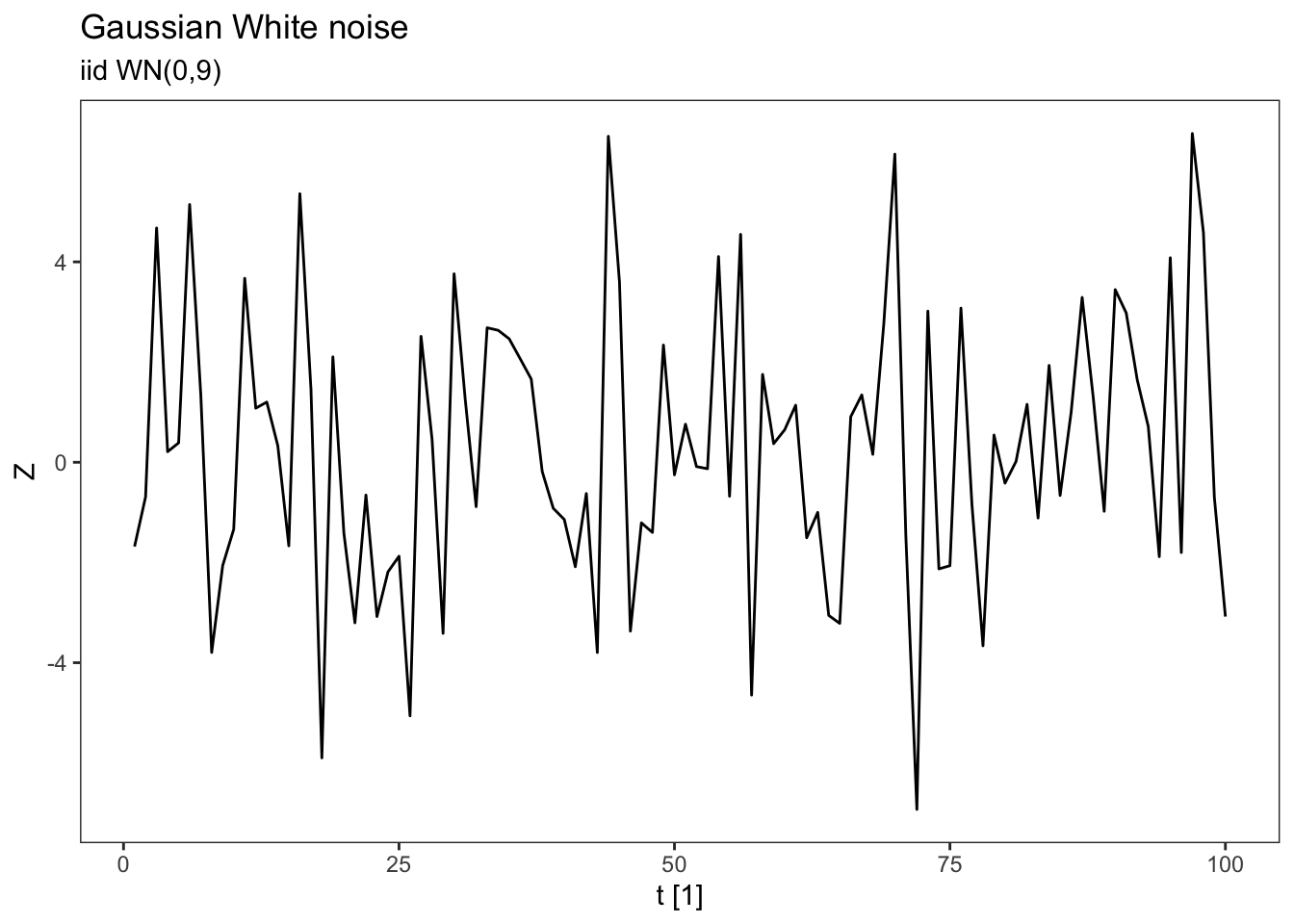
A white noise series is a time series of uncorrelated observations with mean zero and finite variance. We will often write it as Z_t where Z_t \sim \mathrm{WN}(0,\sigma^2). The standard is that the series is uncorrelated, but we may require it to be independent (stronger assumption) and very often normally distributed. In that case we call it iid Gaussian white noise (iid = independent and identically distributed). Notation for this may be Z_t \sim \text{iid}\, \mathrm{WN}(0,\sigma^2). Let us generate a white noise series in R.

library(fpp3)
set.seed(123) # To produce the same output
wn <- tsibble(
  t = 1:100,
  Z = rnorm(100, sd = 3), # Draws from N(0, 3^2) distribution
  index = "t"
)
wn %>%
  autoplot() +
  labs(title = "Gaussian White noise",
       subtitle = "iid WN(0,9)")

Plot variable not specified, automatically selected `.vars = Z`

We can then plot the acf of the series:

wn %>%
  ACF(Z) %>%
  autoplot() +
  labs(title="White noise ACF")

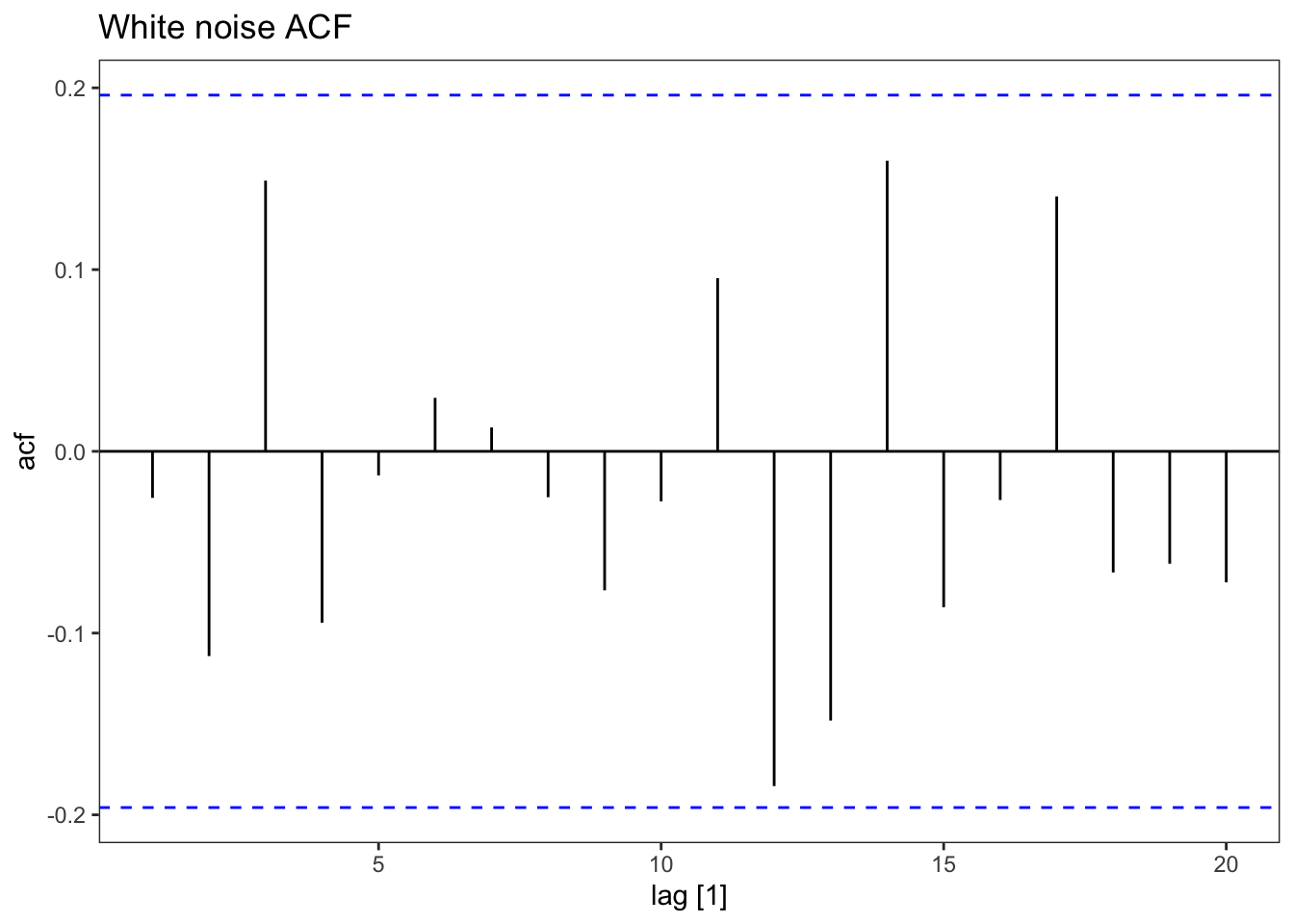
As you can see, all the correlations fall within the confidence bands. The series is uncorrelated. You can also find a similar example in the textbook.