Time series components and Seasonal adjustment

Code

set.seed(1344)
library(tidyverse)
library(fpp3)
dat <- tibble(
  date = seq(as.Date("2015-01-01"), as.Date("2020-12-31"), by = "1 day"),
  t = 1:length(date),
  Tt = 100+9*t/300 + .5*((t-1000)/200)^3+(.87*cos(2*pi*t/1200)+.42*sin(2*pi*t/600))*11,
  St = (.94*cos(2*pi*t/365) -1.2*sin(2* pi*t/365))*13,
  Rt = rnorm(length(date), sd = 15),
  Yt = Tt + St +  Rt
)

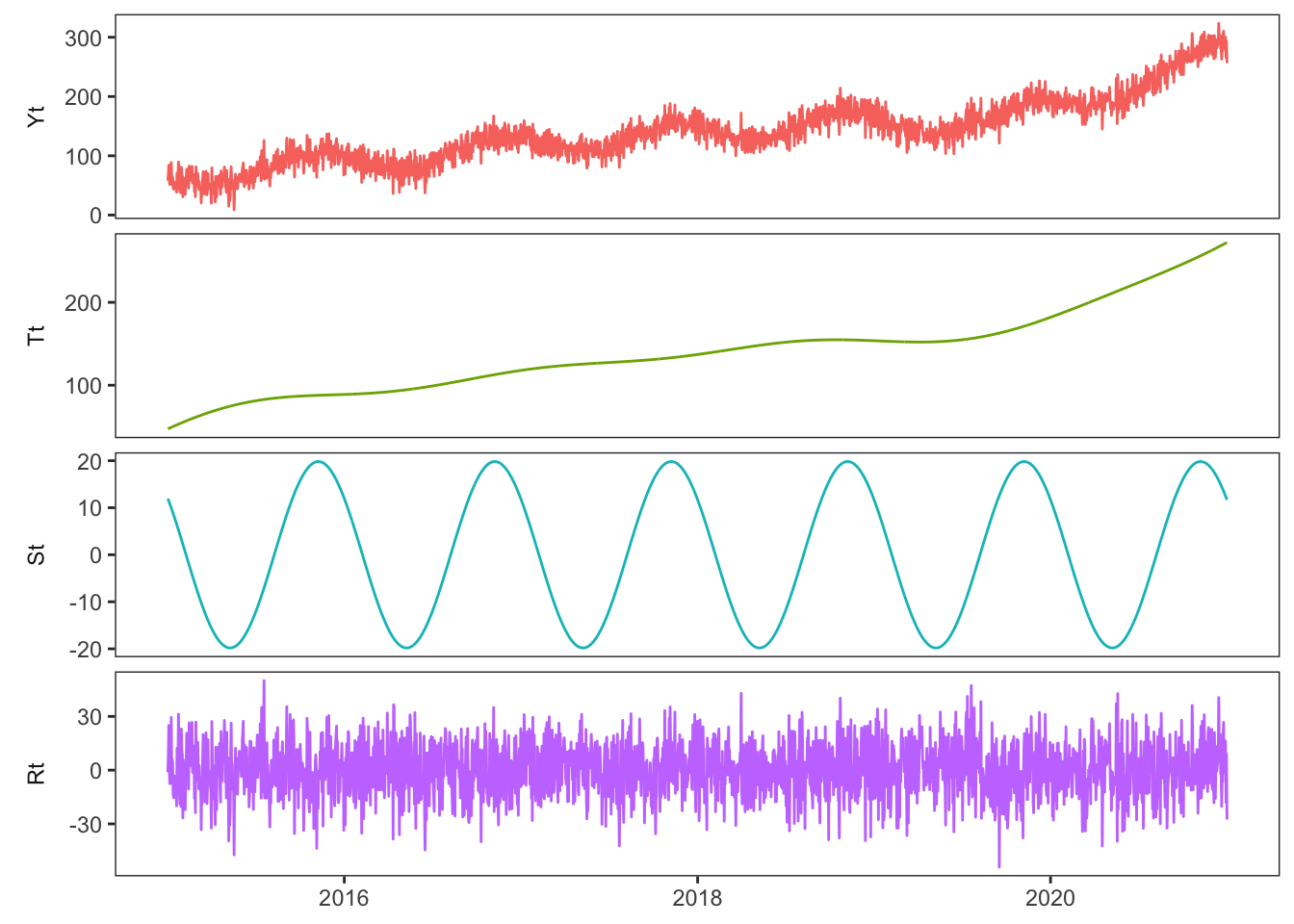
# -- Plotting Y and its components --
dat %>%
  pivot_longer(cols = -c(date,t)) %>%
  mutate(name = factor(name, levels = c("Yt", "Tt", "St", "Rt"))) %>% # to order the panels
  ggplot(aes(x=date, y = value, col = name)) +
  geom_line() + facet_wrap(~name, ncol = 1, scales = "free_y", strip.position = "left") +
  theme(strip.placement = "outside", axis.title = element_blank(), legend.position = "none")

# -- Plotting seasonally adjusted Y --
ggplot(dat, aes(x = date, y = Yt-St)) +
  geom_line() +
  labs(title = "Seasonally adjusted", x = "")