STL: Seasonal and Trend decomposition using Loess

Code

# -- Read in data (see the Moving averages page for details): --
dat <- readxl::read_excel(
  "data/NorwayEmployment_15-74years_bySex.xlsx") %>%
  as_tibble() %>%
  mutate(Quarter = str_replace(Quarter, "K","Q"),
         Quarter = yearquarter(Quarter))
names(dat)[3] <- "Employed"
dat <- dat %>%
  group_by(Quarter) %>%
  summarize(Employed = sum(Employed)) %>%
  as_tsibble(index = Quarter)

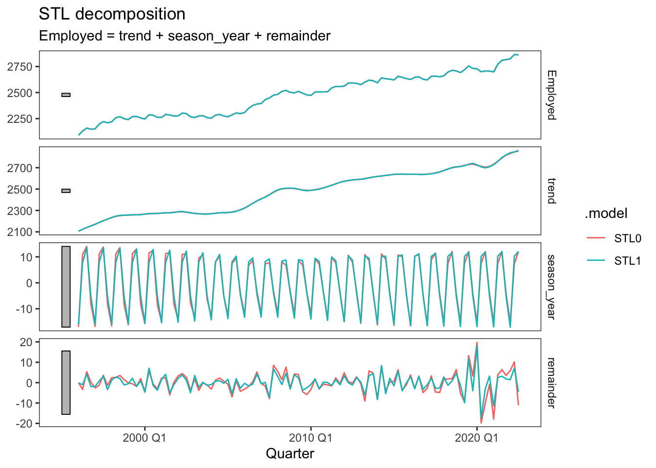
dat %>%
  model(
    STL0 = STL(Employed),
    STL1 = STL(Employed ~ trend(window = 5) + # default 7
                 season(window = 19),         # default 11
               robust = FALSE)
  ) %>%
  components() %>%
  autoplot()