Python

Here we will present some useful python commands relevant for what we want to do in Module 3.

Generate random numbers from a distribution

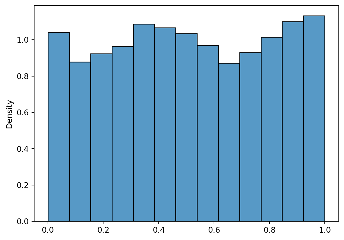
from scipy import stats
import numpy as np
import matplotlib.pyplot as plt
import seaborn as sns
# Generate 2000 random numbers from a uniform distribution: 
x = stats.uniform.rvs(size = 2000)
# Plot histogram of the simulated data: 
sns.histplot(x, stat = "density")
plt.show()
# Add uniform density function to the plot:
sns.histplot(x, stat = "density")
xvalues = np.linspace(0, 1, 2000)
pdf = stats.uniform.pdf(xvalues)
plt.plot(xvalues, pdf, color = "red")
plt.show()

It is often a good idea to set a seed when generating random numbers. This has the benefit that every time you rerun your code, the same random random are generated. If you want a new draw from the distribution, you change the seed and you will get a new set of numbers. Test this out your self using the code below:

np.random.seed(123)
x = stats.uniform.rvs(size = 5)
print(x)
np.random.seed(123)
x = stats.uniform.rvs(size = 5)
print(x)
np.random.seed(124)
x = stats.uniform.rvs(size = 5)
print(x)

[0.69646919 0.28613933 0.22685145 0.55131477 0.71946897]
[0.69646919 0.28613933 0.22685145 0.55131477 0.71946897]
[0.10606491 0.74547148 0.57231354 0.45824118 0.3847059 ]

Monte Carlo simulation: Yatzi

Here we will implement the Yatzi bonus example used in the video here. First, we need a way to simulate the roll of 5 dice and count the number of ones, twos, etc. We could simulate the actual dice, sampling numbers from 1-6 with equal probability. This can be done by the following code:

import numpy as np
np.random.seed(123)
# roll 5 dice:
x1 = np.random.randint(1, 7, size = 5)
print(x1)

[6 3 5 3 2]

We could then count the number of 1 ones and roll the remaining dice.

# Count number of ones:
count_ones1 = np.sum(x1 == 1) 
 # Roll remaining dice:
x2 = np.random.randint(1, 7, size = 5-count_ones1)
print(x2) # Print the outcome
# Count ones in second roll: 
count_ones2 = np.sum(x2 == 1) 
# Roll the remaining dice: 
x3 = np.random.randint(1, 7, size = 5-count_ones1-count_ones2)
print(x3) # Print the outcome
count_ones3 = np.sum(x3 == 1) # count the number of ones
# Calculate the total score: 
score = count_ones1+count_ones2+count_ones3
print(score)

[4 3 4 2 2]
[1 2 2 1 1]
3

This is a bit cumbersome, but it illustrates how one can simulate dice rolls. Since the actual number is not so important for the game, we can rather (as is done in the video), simulate directly the number of ones in the dice roll by simulating from a binomial distribution with sucess probability \(p=1/6\) and \(n=5\) in the first roll, \(n-X_1\) in the second and \(n-X_1-X_2\) in the third.

np.random.seed(321)
from scipy.stats import binom
x1 = binom.rvs(n=5, p=1/6, size = 1) # First roll
x2 = binom.rvs(n=5-x1, p=1/6, size = 1) # Second roll 
x3 = binom.rvs(n=5-x1-x2, p=1/6, size = 1) # Second roll 
print("After first roll:",   x1)
print("After second roll:",  x1+x2)
print("Score of the round:", x1+x2+x3)

After first roll: [2]
After second roll: [2]
Score of the round: [4]

This was one round of Yatzi, where the score is just the number of equal dice rolls or you could think of it as the round where we collect ones. Let’s make this a function. We also add the argument number, which is the number we are collect in the specific round.

from scipy.stats import binom

def play_round(number, n=5, p=1/6):
    x1 = binom.rvs(n=n, p=p, size=1)[0]          # First roll
    x2 = binom.rvs(n=n - x1, p=p, size=1)[0]     # Second roll
    x3 = binom.rvs(n=n - x1 - x2, p=p, size=1)[0]  # Third roll
    return (x1 + x2 + x3)*number
  
# Play round collecting ones:
print(play_round(1))

2

and use it to play a full game:

def play_game():
    total_score = 0
    for i in range(1, 7):
        total_score += play_round(i) # add the next round to total score
    return total_score
print("Game score:", play_game())
# No bonus this round.

Game score: 34

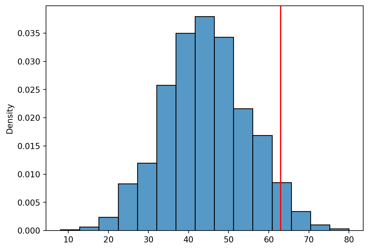
We can now run many-many games. That is, we are ready to do a Monte Carlo simulation of the game.

# Play 10,000 games: 
scores = np.array([play_game() for _ in range(10_000)])

Having played 10,000 games, we can estimate the expected score:

m = scores.mean() 
print("Expected score: ", m)

Expected score:  44.237

The probability of achieving the bonus requirement (total score \(\le 63\)):

bonus_prob = np.mean(scores>=63)
print("Expected score: ", bonus_prob)

Expected score:  0.0432

Or plot the distribution of the scores:

sns.histplot(scores, bins = 15, stat = "density")
plt.axvline(63, color = "red")
plt.show()

Bootstrap

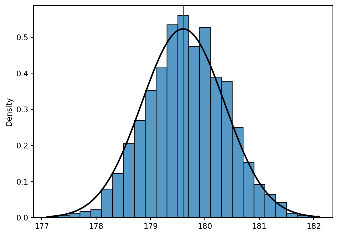
We consider the same height measurements of ten 20-year old male athletes as used in the video on the bootstrap. We can first confirm that the sample mean is 179.6 and the standard deviation is 2.41. This the standard error of the sample mean estimator being \(\approx \sigma/\sqrt{n}= 2.41/\sqrt{10}=0.76\).

import pandas as pd
import math
numbers = [183, 179, 179, 183, 178, 176, 182, 177, 180, 179]
vector = pd.Series(numbers)
print(vector.mean())
print(vector.std())
print(vector.std()/math.sqrt(10))

179.6
2.412928142780514
0.7630348761506397

To sample randomly from this vector of observations, we can use the following code:

np.random.seed(1234)
newsample = vector.sample(3, replace = False)
print(newsample)

7    177
2    179
9    179
dtype: int64

As you can see from the output, I have sampled 3 heights from the vector. Here I have sampled without replacement, so I know that these are three different observations selected at random. I set a seed to get the same three each time I run the code.

Now, say we want to use the bootstrap method to find the sampling distribution of the sample mean estimator from just this one sample of ten observations. We then pretend that the data we have (the ten observations) is our population, and we repeatedly sample from the vector with replacement. For each new sample we calculate the average value and the vector containing many such mean value (boot_means) is treated as observations of the sample mean estimators for multiple samples. We can summarize the sampling distribution by e.g. considering the standard deviation of the boot_means. This should be close to the \(\sigma/\sqrt{n}\) value that we found above, due to the central limit theorem and the fact that we are considering a mean estimator here.

np.random.seed(123)
bootstrap_samples = 2000
boot_means = np.zeros(bootstrap_samples)
for b in range(0, bootstrap_samples) : 
    boot_sample = vector.sample(len(vector), replace = True)
    boot_means[b] = boot_sample.mean()
print(boot_means.std())

0.7292611997768702

We can also plot the sampling distribution:

from scipy.stats import norm
# Histogram of sampling distribution
sns.histplot(boot_means, stat = "density", binwidth = .2)
plt.axvline(x=vector.mean(), color = "red")

# Add normal density curve: 
x = np.linspace(min(boot_means), max(boot_means), 500)
mu = np.mean(vector)
sigma = np.std(vector, ddof=1)/np.sqrt(10)

plt.plot(x, norm.pdf(x, mu, sigma), color="black", linewidth=2)

plt.show()

Note that the black curve is based on the normal approximation (central limit theorem). Quite a good fit!

Now, let us consider a slightly larger dataset. This example is from the python supplement to the textbook. Here we imagine that the full NHANES dataset is our population. We pull out a sample of size 100 as our “original sample”. We then bootstrap the sampling distribution of the mean height. Here, we are not interested in the mean or the standard deviation, but the 2.5 and 97.5 percentiles. This gives the central interval containing 95% of the population.

from nhanes.load import load_NHANES_data
import pandas as pd
nhanes_data = load_NHANES_data()
adult_nhanes_data = nhanes_data.query('AgeInYearsAtScreening > 17')
adult_nhanes_data = adult_nhanes_data.dropna(subset=['StandingHeightCm']).rename(columns={'StandingHeightCm': 'Height'})

num_runs = 5000
sample_size = 100

# Take a sample for which we will perform the bootstrap

nhanes_sample = adult_nhanes_data.sample(sample_size)

# Perform the resampling

bootstrap_df = pd.DataFrame({'mean': np.zeros(num_runs)})
for sampling_run in range(num_runs):
    bootstrap_sample = nhanes_sample.sample(sample_size, replace=True)
    bootstrap_df.loc[sampling_run, 'mean'] = bootstrap_sample['Height'].mean()

# Compute the 2.5% and 97.5% percentiles of the distribution
bootstrap_ci = np.percentile(bootstrap_df['mean'], [2.5, 97.5])
print("Bootstrap 95% CI:", bootstrap_ci)

# Normal approximation:
sample_mean = nhanes_sample["Height"].mean()
sample_std = nhanes_sample["Height"].std()/np.sqrt(sample_size)
CLT_ci = norm.ppf([0.025,0.975], sample_mean, sample_std)
print("Normal approximation 95% CI:", CLT_ci)

Bootstrap 95% CI: [165.458975 168.960025]
Normal approximation 95% CI: [165.4873607 168.9686393]

In this case, we expect the two approaches to give similar results, and this is also what we get here.