Hypothesis testing in Python

In any given hypothesis testing situation, we need to decide

Inference About One Population

Test Null Hypothesis Test Statistic Distribution Under \(H_0\) Comments
Test for a population mean \(H_0: \mu = \mu_0\) \(T = \frac{\bar X - \mu_0}{s / \sqrt{n}}\) t-distribution, \(n-1\) df One- or two-sided
Test for a population variance \(H_0: \sigma = \sigma_0\) \(\chi^2 = \frac{(n-1)s^2}{\sigma_0^2}\) \(\chi^2\)-distribution, \(n-1\) df One- or two-sided; skewed
Test for a population proportion \(H_0: p = p_0\) \(Z = \frac{\hat p - p_0}{\sqrt{p_0(1-p_0)/n}}\) Standard normal One- or two-sided

Inference About Two Populations

Test Null Hypothesis Test Statistic Distribution Under H₀ Comments
Equal means (independent, equal variances) \(H_0: \mu_1 = \mu_2\) \(T = \frac{\bar X_1 - \bar X_2}{\sqrt{s_p^2(1/n_1 + 1/n_2)}}\) t-distribution, \(n_1 + n_2 - 2\) df Pooled variance
Equal means (independent, unequal variances — Welch) \(H_0: \mu_1 = \mu_2\) \(T = \frac{\bar X_1 - \bar X_2}{\sqrt{s_1^2/n_1 + s_2^2/n_2}}\) Welch’s t-distribution: \(\text{df}=\frac{(S_1^2/n_1+S_2^2/n_2)^2}{\frac{(S_1^2/n_1)^2}{n_1-1}+\frac{(S_2^2/n_2)^2}{n_2-1}}\) Robust to unequal variances
Equal means (paired samples) \(H_0: \mu_D = 0\) \(T = \frac{\bar D}{s_D / \sqrt{n}}\) t-distribution, \(n-1\) df Use differences
Equal variances \(H_0: \sigma_1^2 = \sigma_2^2\) \(F = \frac{s_1^2}{s_2^2}\) F-distribution, \((n_1-1, n_2-1)\) df Place larger variance in numerator
Equal proportions \(H_0: p_1 = p_2\) \(Z = \frac{\hat p_1 - \hat p_2}{\sqrt{\hat p(1-\hat p)(1/n_1 + 1/n_2)}}\) Standard normal Uses pooled proportion \(\hat p\)

Paired t-test

We have measured the weight of five people before and after a diet.

\[H_0: \mu_\text{before}=\mu_\text{after}\quad \text{vs}\quad H_A: \mu_\text{before} >\mu_\text{after}.\]

import numpy as np
from scipy import stats
before = np.array((85, 76, 72, 92, 79)) # weight in kg
after  = np.array((78, 73, 83, 89, 71)) 
paired_test = stats.ttest_rel(before, after, alternative="greater")
print(paired_test)
TtestResult(statistic=np.float64(0.5872202195147035), pvalue=np.float64(0.29430108085972617), df=np.int64(4))

As you can see, the default print of the test object is not very pretty. Let us format the printout a bit nicer:

print(f"Paired t-test (one-sided)\n"
      f"-------------------------\n"
      f"t-statistic : {paired_test.statistic:.4f}\n"
      f"p-value     : {paired_test.pvalue:.4f}\n")
Paired t-test (one-sided)
-------------------------
t-statistic : 0.5872
p-value     : 0.2943

This test is equivalent to doing a one-sample t-test on the weight difference. \[H_0: \mu_d=0\quad \text{vs}\quad H_A: \mu_d >0.\]

diff = before-after
onesample_test = stats.ttest_1samp(diff, popmean = 0, 
                                   alternative = "greater")
print(onesample_test)
print(f"One-sample t-test (one-sided)\n"
      f"-------------------------\n"
      f"t-statistic : {onesample_test.statistic:.4f}\n"
      f"p-value     : {onesample_test.pvalue:.4f}\n")
TtestResult(statistic=np.float64(0.5872202195147035), pvalue=np.float64(0.29430108085972617), df=np.int64(4))
One-sample t-test (one-sided)
-------------------------
t-statistic : 0.5872
p-value     : 0.2943

As you can see, the test statistics and corresponding p-values are equal. Since the p-value is high, the evidence against the null-hypothesis is weak, and for a given significance level (say 10%), we would not reject the null of change in expected weight following the diet. The expected weight is equal before and after the diet. Five people is very few for testing a diet, so we could suggest that the investigators collect more data.

Proportions test - one sample

To evaluate whether an observed proportion differs from a specified benchmark, we can carry out a one-sample test of proportions in Python.

As an example, let’s say \(p\) is the probability of heads for a given coin. We want to test if the coin is fair, i.e.

\[H_0: p = 0.5\quad \text{vs}\quad H_A:p\neq 0.5\] with a significance level of 5%. We toss the coin ten times and observe 4 heads.

from scipy import stats
from statsmodels.stats.proportion import proportions_ztest
prop_test = proportions_ztest(count = 4,
                  nobs = 10,
                  value = 0.5,
                  alternative = "two-sided")
print(prop_test)
(np.float64(-0.6454972243679027), np.float64(0.5186050164287257))

This test is based on a normal approximation of the binomial distribution. We could do the corresponding exact test, using a binomial test:

stats.binomtest(4, 10, 0.5, alternative = "two-sided")
BinomTestResult(k=4, n=10, alternative='two-sided', statistic=0.4, pvalue=0.75390625)

A common rule of thumb is that when \(np>5\), the approximation is good. In this case we are exactly on this common threshold.

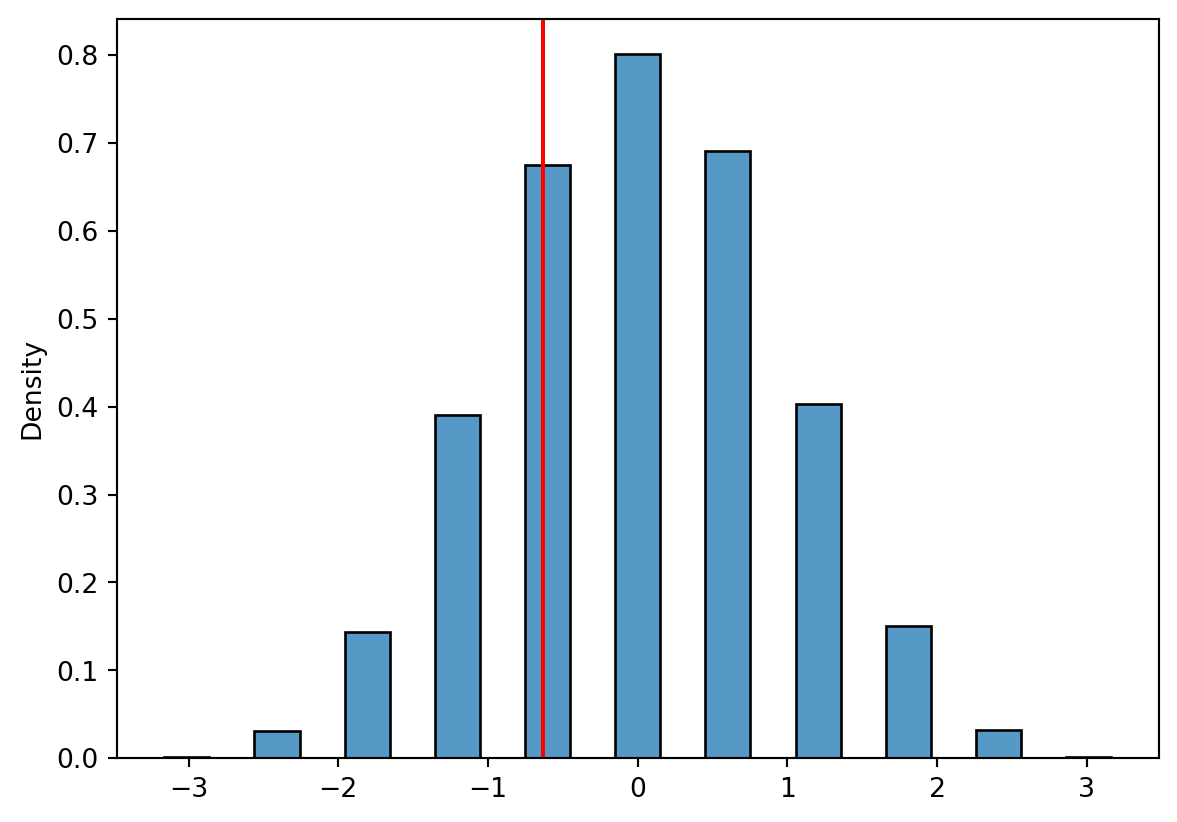
Another alternative is to use a bootstrap approach for testing.

np.random.seed(12345)
import seaborn as sns
import matplotlib.pyplot as plt
sample_size = 10
count = 4
phat = stats.binom.rvs(n=sample_size, p = 0.5, size = 10000)/sample_size
z = (phat-0.5)/np.sqrt(0.5*0.5/sample_size)
z_stat = (count/sample_size - 0.5)/np.sqrt(0.5*0.5/sample_size)
sns.histplot(z, binwidth = .3, stat = "density")
plt.axvline(x=z_stat, color = "red")
plt.show()
print("Statistic: ", np.round(z_stat,3),
      "\nNumber exceeding: ", (z>z_stat).sum(),
      "\nPercentage: ", np.round((z>z_stat).mean()*100,3),"%")

Statistic:  -0.632 
Number exceeding:  6261 
Percentage:  62.61 %

Two-saple test of proportions

Instead of comparing a proportion to a benchmark value, we can compare proportions between two groups.

Example: A web store wants to test whether changing the color of the “buy” button effects sales (e.g. increases the rate of clicking “buy”). When customers load the website, they assign a 50% chance that the customer sees a blue (group A) or green (group B) buy button. Does changing the color from blue to green increase the rate of customers clicking “buy”?

\[H_0: p_A=p_B\quad \text{vs}\quad p_A < p_B.\] We can accept a high significance level here, since we are not afraid of making type I error (incorrectly rejecting a true null hypothesis). Let us use \(\alpha = 10\%\).

Group Sample size Clicks Rate
A (blue button) 2359 543 23%
B (green button) 2523 606 24%

The observed rate is higher for green button, but lets perform the test in Python:

from statsmodels.stats.proportion import test_proportions_2indep
test = test_proportions_2indep(count1=543, 
                               nobs1=2359,
                               count2=606,
                               nobs2=2523,
                               value=0,
                               method="wald",
                               compare='diff',
                               alternative='smaller')
print(test)
statistic = -0.8241828933434447
pvalue = 0.2049178227694594
compare = diff
method = wald
diff = -0.010007969075350343
ratio = 0.9583331584536157
odds_ratio = 0.9458744057225107
variance = 0.0001474499797394375
alternative = smaller
value = 0
tuple = (np.float64(-0.8241828933434447), np.float64(0.2049178227694594))

The experimental setup described above if often called an AB-test. An A/B test is any randomized experiment comparing two versions (A and B) of something to see which performs better on some outcome.

We can do the test also “by hand”. The test statistic is \[Z=\frac{\widehat p_A-\widehat p_B}{\text{SE}},\] where \[ \widehat p_\text{pool} = \frac{\text{Total clicks}}{\text{Total customers}} = \frac{545+606}{2359+2523}=23.58\% \] and \[\text{SE}=\sqrt{\widehat p_\text{pool}(1-\widehat p_\text{pool})(\frac1{n_1}+\frac1{n_2})}=0.01216\] Thus, \[ Z = \frac{0.23-0.24}{0.01216}=-0.82 \] Note that, if the alternative hypothesis is true, \(p_A\) is smaller than \(p_B\), making \(Z\) negative. So we reject the null hypothesis for small values of Z (i.e. large negative values). To find the p-value,

\[P(Z\le z)=P(Z\le -0.82) = 0.2061\] based on

from scipy.stats import norm
print(round(norm.cdf(-0.82),4))
0.2061

With \(\alpha = 10\%\) we would not reject the null hypothesis, since the p-value exceeds the significance level. The evidence does not suggest any difference between the clicking rates for green versus blue buying buttons.